For many developers, GPU programming feels like a dark art. We know that under the hood of every major AI breakthrough lies a massive cluster of GPUs, churning through math at unimaginable speeds. But actually writing the code to control that hardware? That often feels like a barrier too high to cross.
I recently dove into the basics of CUDA C++, and the biggest challenge wasn’t the syntax; it was the mental shift.
If you are coming from standard CPU programming (Python, C++, Java), you are used to thinking sequentially. You have a fast race car (the CPU), and you drive it around a track completing tasks one by one.
GPU programming requires a different approach. Instead of a race car, you have an army of thousands of ants. Each ant is slow and can only do one very specific task, but they all work at the exact same time.
The best way to understand this shift is through the “Hello World” of high-performance computing: Matrix Multiplication.
The CPU Mindset vs. The GPU Mindset
To multiply two matrices (C = A times B) on a CPU, you write three nested for loops. You calculate C[0][0], then C[0][1], and so on, linearly.
On a GPU, we flip the script. We don’t write loops to iterate over the whole matrix. We write code for exactly one output pixel.
We then tell the GPU: “Spawn millions of threads, and have every single thread execute this same piece of code simultaneously.”
The Kernel
This single piece of code is called the Kernel. Here is the “naive” implementation of a Matrix Multiplication kernel in CUDA C++.
Notice there are no outer loops defining rows and columns. Instead, the thread has to figure out “Who am I?” using built-in hardware variables.
C++
__global__ void matrix_multiplication_kernel(const float* A, const float* B, float* C, int M, int N, int K) {
    // 1. Find Identity: Who am I?
    // Each thread calculates its unique global (row, col) coordinate.
    int row = blockIdx.y * blockDim.y + threadIdx.y;
    int col = blockIdx.x * blockDim.x + threadIdx.x;

    // 2. Safety Check: Am I inside the matrix?
    // Grids are launched in fixed-size blocks (e.g., 16x16).
    // If the matrix size isn’t a perfect multiple, some threads hang off the edge.
    // We must ensure they don’t access invalid memory.
    if (row < M && col < K) {
        float sum = 0.0f;

        // 3. The Work: Dot Product
        // Sweep across Row ‘row’ of A and Column ‘col’ of B
        for (int n = 0; n < N; n++) {
            // Note the flattened 1D memory access math
            sum += A[row * N + n] * B[n * K + col];
        }

        // 4. Write Result
        C[row * K + col] = sum;
    }
}
Visualizing the Grid
The magic happens in how we organize those thousands of threads. CUDA uses a hierarchy:
Threads: The individual workers.
Blocks: Groups of threads that work together (think of a 16 times 16 square tile of threads).
Grid: The entire collection of blocks needed to cover your data.
On the host (CPU) side, we define this geometry before launching the kernel. We define a “tile” size (e.g., 16*16 threads) and then calculate how many tiles we need to cover the dimensions of our matrix.
If you imagine your matrix as a large kitchen floor, threadsPerBlock is the size of the tile you are using, and blocksPerGrid is the blueprint telling you how many tiles you need to buy to cover the floor.
Why This Matters
This “naive” implementation is just the stepping stone. Real-world CUDA optimization involves using Shared Memory (a user-managed cache on the GPU) to prevent threads from constantly reaching out to slow global memory.
But understanding this fundamental grid structure is the prerequisite to everything else in accelerated computing, whether you are running inference on an Nvidia T4 in Google Colab or exploring new languages like Mojo designed to bridge the gap between Python’s ease of use and CUDA’s raw speed.
The learning curve is steep, but the view from the top, where you can execute trillions of operations per second, is worth it.
Here’s my recently recorded YouTube Video :


